Searching For Duplicates With Excel
I was speaking to someone this week about finding duplicates in lists which got me thinking about how that might be done in Excel. From the top of my head (why there, nobody knows), I could think of 4 ways in which you could identify them, so let’s zip through what I could come up with.
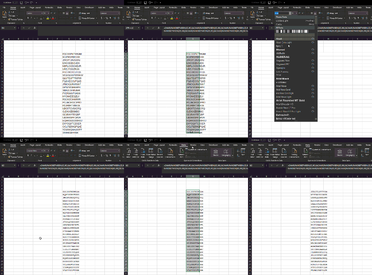
Here’s an example of the list I will be using:

Manually
Once your list is pasted into Excel, the first thing you might notice is that the list is using a variable width font. Fix that by selecting the list, then changing to something like Courier New which is monospaced.
Next, sort the list, and you should be able to identify any that are the same fairly easily as they will be the same length and the strings more uniform.

- Advantage - Simple to do.
- Disadvantage - Not much fun if the list is large.
Counting Duplicates
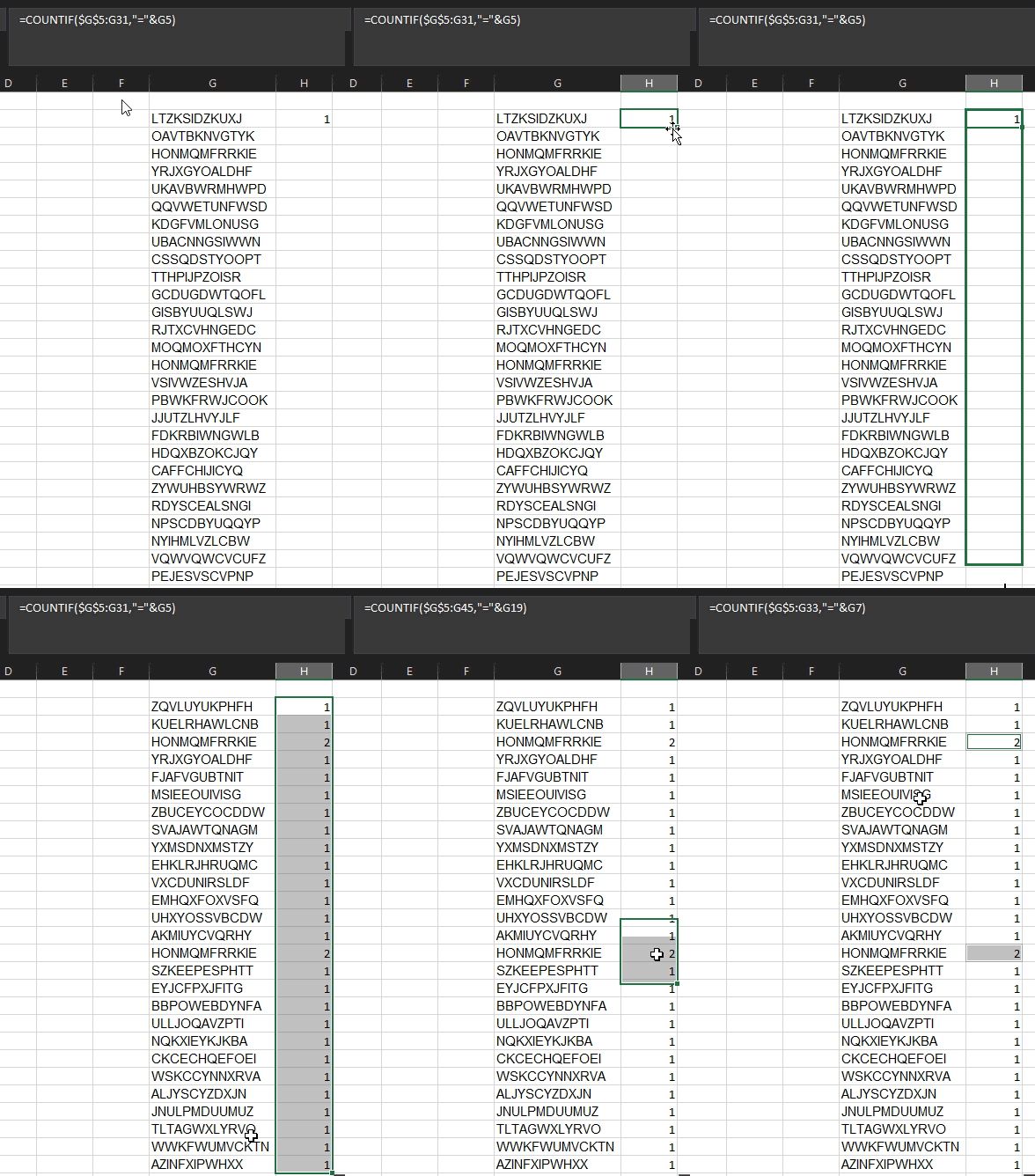
There’s a useful function in Excel called COUNTIF. The first parameter is the range you are examining, and the second, the test you want to apply to each cell.
The format of this test is a string preceded with an equals sign, so what we need to do is write something like:
1 | =COUNTIF(A:A, "=STRINGTOSEARCHFOR") |
That will search in the A column for any cells that match “STRINGTOSEARCHFOR” and sum up how many it finds. To accomplish what we want though, we need to keep changing the STRINGTOSEARCHFOR and that is done by making the test dynamic.
1 | =COUNTIF(A:A, "="&A1) |
In this example, we are saying, count all the values in the A column that match what is in A1. We then drag the formula down through the cells with Excel changing the formula to A2, A3, etc. and look for any which return more than 1. Why that and not something else? Well, there will alway be at least 1, right?

- Advantage: easy to understand
- Disadvantage: another stage needed to highlight the duplicates (e.g. filters).
Checking Your Neighbour
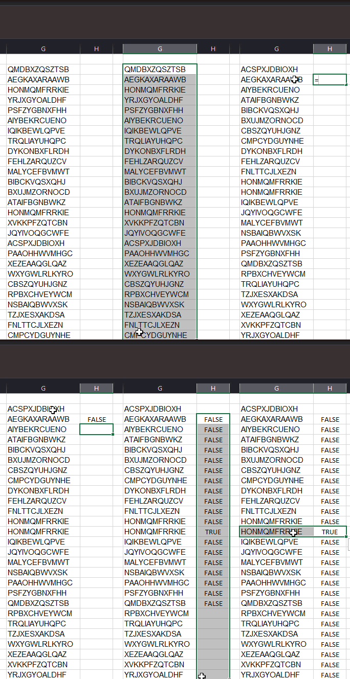
For this method, you need to select your list, then sort it using the A-Z tool.
Next, in the column along side it, starting at the second entry, use something like this formula:
1 | = A1 = A2 |
Lastly, drag the formular down through the range to the bottom of the list.
What you will end up with is a bunch of TRUE or FALSE values. TRUE indicates a match (or duplicated) and FALSE, the opposite.

- Advantage and Disadvantage: Much like the COUNTIF example.
Using Highlight Duplicates Feature
Saving the best till last.
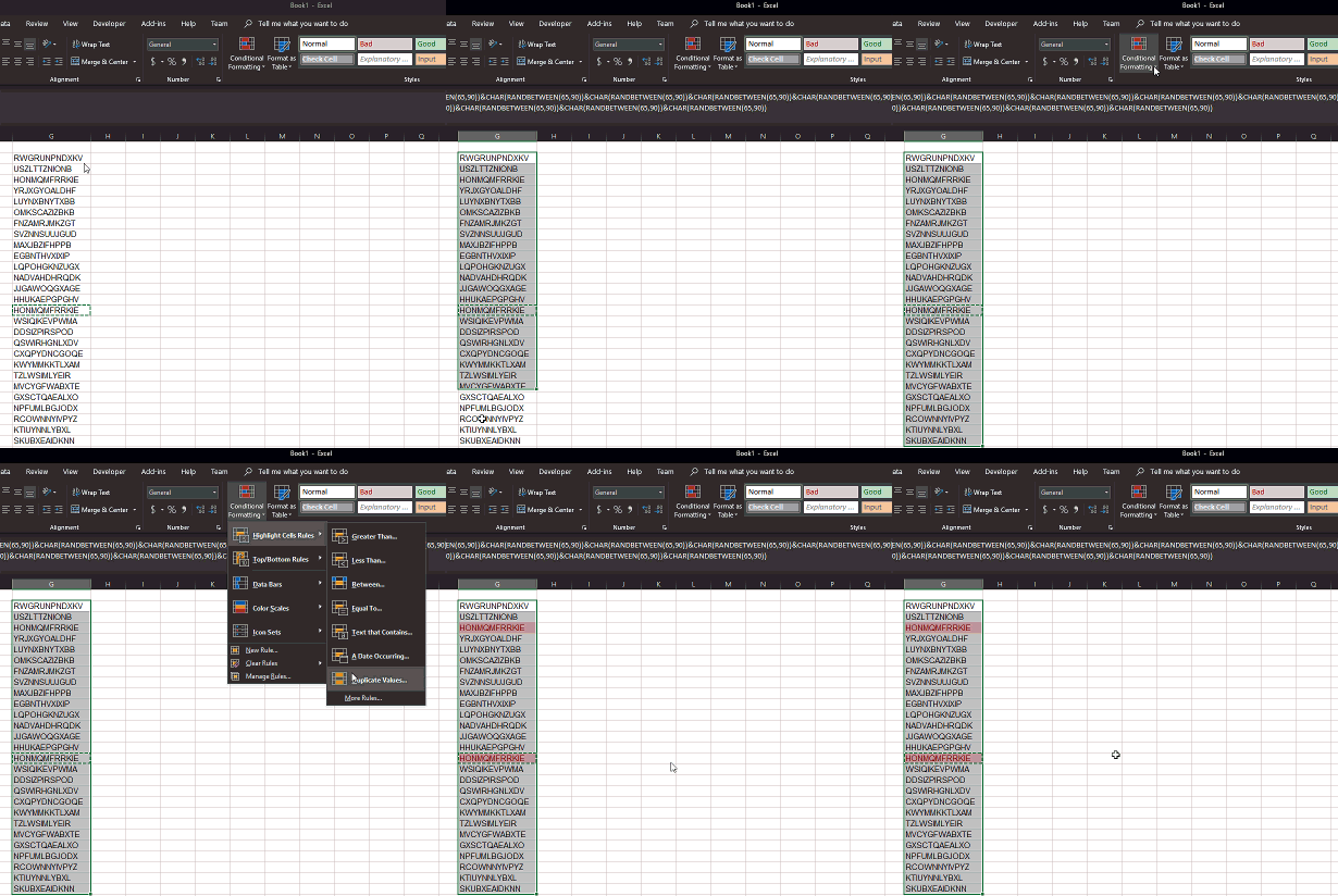
For this, if you have a new enough version of Excel, you can get the application to highlight any duplicates.
- Change to the Home menu ribbon
- Select the list
- Click on Conditional Formatting
- Click on Highlight Cell Rules
- Click on Duplicate Values…
- Click OK.
Any cells that are duplicates will be highlighted.

- Advantage: A few clicks and it’s done.
- Disadvantage: Err…none!
Hi! Did you find this useful or interesting? I have an email list coming soon, but in the meantime, if you ready anything you fancy chatting about, I would love to hear from you. You can contact me here or at stephen ‘at’ logicalmoon.com